Your MAU is not your load: capacity math for voice AI at scale

The first capacity meeting for a voice assistant always starts the same way. Someone puts a big number on the slide, “we expect a million users”, and everyone in the room quietly starts multiplying it by GPUs. I’ve learned to stop that multiplication early. It’s the wrong number to multiply.

This post is the back-of-the-envelope method I use to go from a user count to hardware. None of it is secret. It’s Little’s law, some memory arithmetic and a latency budget. But doing it in this order keeps a team from over-buying by 10× or, worse, launching on a cluster that falls over at 8 p.m. on day one.

The numbers below are an illustrative example, not any real system. Swap in your own.

Start from the experience, not the hardware

Voice is unforgiving. In a text chat, a 3-second wait feels fine. In a conversation, it feels like the other person has walked away. Studies of turn-taking across ten languages put the typical gap between speakers at around 200 ms (Stivers et al., PNAS 2009). We can’t hit that with a pipeline of models, but it tells you which direction “good” is.

So before any GPU math I write down a voice-to-voice budget: the time from the moment the user stops talking to the moment they hear the first syllable back.

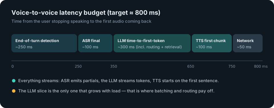A budget of about 800 ms. Every stage streams, and only the LLM slice grows with load.

Two things fall out of this picture straight away.

First, everything has to stream. If ASR waits for the full utterance, the LLM waits for the full transcript and TTS waits for the full answer, you’ve spent your budget three times over. ASR emits partial hypotheses, the LLM streams tokens, and TTS starts speaking as soon as the first sentence is complete.

Second, end-of-turn detection is the biggest single slice, and it isn’t a GPU problem at all. A plain silence timeout of 700 ms makes the bot feel slow. One of 200 ms makes it interrupt people who pause to think. A small model that predicts “is this turn finished?” from the audio and the partial text is one of the cheapest latency wins there is.

The LLM’s slice, time-to-first-token (TTFT), is the only one that degrades as traffic grows. That’s where the rest of this post goes.

From monthly users to concurrent sessions

Here’s the trap. MAU tells you how many people exist. Your GPUs only care how many are talking right now.

The bridge is Little’s law (Little, 1961), which holds for any stable queueing system:

$$L = \lambda \, W$$

$L$ is the average number of things in the system, $\lambda$ is the arrival rate and $W$ is how long each one stays. It doesn’t care about distributions, which is exactly why it’s useful this early.

Let’s walk the example:

Step	Assumption	Result
Monthly active users	given	1,000,000
Daily active users	DAU/MAU = 20%	200,000
Sessions per day	1.5 per DAU	300,000
Peak-hour share	10% of daily sessions	30,000 sessions/hour
Arrival rate $\lambda$	30,000 / 3,600 s	≈ 8.3 sessions/s
Session length $W$	4 minutes	240 s
Live sessions $L$	$\lambda W$	≈ 2,000

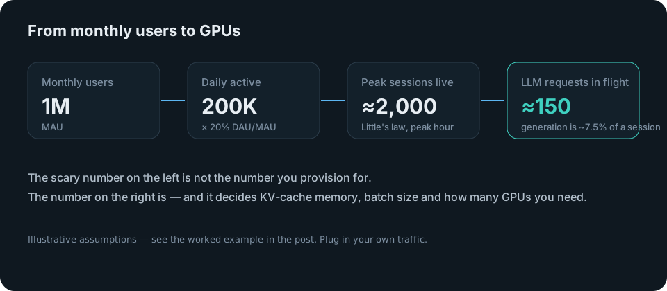From the scary number to the one you actually provision for.

A million users became about two thousand live conversations at the busiest hour of the day. That’s still a lot, but it’s a different conversation from “a million”.

It gets smaller again. A live session is mostly not using the LLM. The user is speaking, the bot is speaking, someone is thinking. Suppose a turn cycle takes ~20 s, and the LLM spends ~1.5 s of that actually generating. Then the LLM duty cycle is

$$\rho_{\text{LLM}} = \frac{1.5}{20} = 7.5\%, \qquad L_{\text{LLM}} \approx 2{,}000 \times 0.075 = 150 .$$

About 150 requests in flight. That’s the number that sizes your LLM tier. ASR is different: it listens whenever the user speaks, so its duty cycle is much higher. That’s one reason I almost always scale ASR, LLM and TTS as separate pools rather than one fat pod.

How much memory do 150 requests need?

Model weights are the part everyone remembers. The part that bites is the KV cache: for every token in every active request, each layer stores a key and a value vector.

$$\text{KV bytes per token} = 2 \times n_{\text{layers}} \times n_{\text{kv\_heads}} \times d_{\text{head}} \times \text{bytes per value}$$

Take an 8B model in the Llama 3 shape: 32 layers and grouped-query attention with 8 KV heads of dimension 128 (Llama 3 paper, Table 3), in bf16 (2 bytes):

$$2 \times 32 \times 8 \times 128 \times 2 = 131{,}072 \text{ bytes} = 128\ \text{KiB per token}.$$

That sounds tiny until you multiply. A voice agent with a system prompt, tool definitions, retrieved context and conversation history easily sits at 4,000 tokens:

$$4{,}000 \times 128\ \text{KiB} \approx 0.5\ \text{GiB per request}, \qquad 150 \times 0.5 \approx 75\ \text{GiB}.$$

On an 80 GB GPU, the bf16 weights take about 16 GB. After activations and framework overhead you have maybe 55–60 GB for KV. So KV alone needs two GPUs before we’ve even asked whether they’re fast enough.

Three things change this picture a lot:

1. Prefix caching. In an agent, the system prompt and tool schemas are identical across users. Cache their KV once and share it. If 2,500 of those 4,000 tokens are a shared prefix, per-request memory drops by more than half.
2. Paged KV. Allocating KV in fixed blocks, as vLLM’s PagedAttention does, removes the fragmentation that otherwise wastes a big chunk of memory.
3. Shorter context by design. Summarise old turns. Retrieve less, but better. The cheapest token is the one you never put in the prompt.

Are they fast enough?

At small batch sizes, decoding is limited by memory bandwidth, not FLOPs. Each step has to read every weight once, plus the KV of every sequence in the batch. A useful first estimate:

$$\text{steps/s} \approx \frac{\text{memory bandwidth}}{\text{weight bytes} + \text{KV bytes read per step}}$$

Take an H100 SXM, with 3.35 TB/s of memory bandwidth. Add 16 GB of weights and a batch of 75 requests averaging 2,000 tokens of live context ($75 \times 2{,}000 \times 128\ \text{KiB} \approx 20\ \text{GB}$). That gives you on the order of 90 decode steps per second. Every sequence in the batch advances one token per step, so each stream sees ~90 tokens/s. That’s far faster than anyone can listen, and it leaves real headroom.

This is why continuous batching matters so much. Requests join and leave the batch at every step, instead of waiting for the slowest one, so you keep the GPU near this bandwidth ceiling under real, uneven traffic.

So the rough answer for this example is 2–3 GPUs for the LLM tier at peak, plus headroom for failover. That’s very different from the number people start multiplying in that first meeting.

Make most requests cheaper

The biggest scaling lever isn’t hardware. It’s not sending every turn to the biggest model.

In a multi-agent setup, a small, fast router decides what each turn needs. “Turn off the bedroom light” needs a tool call, not a 70B model reasoning about it. Only the genuinely open-ended turns go to the large model. If 70% of traffic can be served by a model a quarter of the size, the expensive tier only sees 30% of $L_{\text{LLM}}$.

Tools behind a standard interface (I like MCP for this) keep the agents themselves small. They decide what to do, and deterministic code does it.

Plan for the tail, not the average

Everything above is about averages. Users experience the tail. Two habits help:

• Budget at p95, not the mean. A queue that’s 80% utilised has far longer waits than one at 60%. Wait time blows up as utilisation approaches 1, roughly like $\frac{\rho}{1-\rho}$ for the textbook M/M/1 queue. I aim to keep LLM pools around 60–70% at the expected peak.
• Degrade gracefully. When the big model is saturated, fall back to the small one with a shorter answer, rather than making people wait. A slightly worse answer now beats a perfect one in four seconds.

The checklist I actually use

1. Write the voice-to-voice latency budget first.
2. Convert MAU → live sessions → in-flight LLM requests with Little’s law and a duty cycle.
3. Size KV-cache memory per request, then apply prefix caching and context limits.
4. Check decode speed against memory bandwidth at your target batch size.
5. Route cheap turns to cheap models, and scale ASR, LLM and TTS as separate pools.
6. Leave headroom for the tail, and measure p95 in production, every day.

None of this replaces load testing. But it gets you to the right order of magnitude before you spend money, and it gives the load test a hypothesis to prove wrong.

References

• Stivers, T. et al. (2009). Universals and cultural variation in turn-taking in conversation. PNAS, 106(26).
• Little, J. D. C. (1961). A proof for the queuing formula L = λW. Operations Research, 9(3).
• Llama Team, AI @ Meta (2024). The Llama 3 Herd of Models. arXiv:2407.21783 — model shapes (layers, KV heads).
• Kwon, W. et al. (2023). Efficient Memory Management for Large Language Model Serving with PagedAttention. SOSP 2023 — vLLM, paged KV cache and continuous batching.
• NVIDIA. H100 Tensor Core GPU specifications — memory bandwidth.
• M/M/1 queue — waiting time versus utilisation.
• Model Context Protocol — tool interface for agents.

The traffic figures (1M MAU, DAU/MAU, session length, peak share) are illustrative assumptions, not measurements from any real system.